PRECOG
Please read carefully to understand the data structure and its evaluation
Prediction example
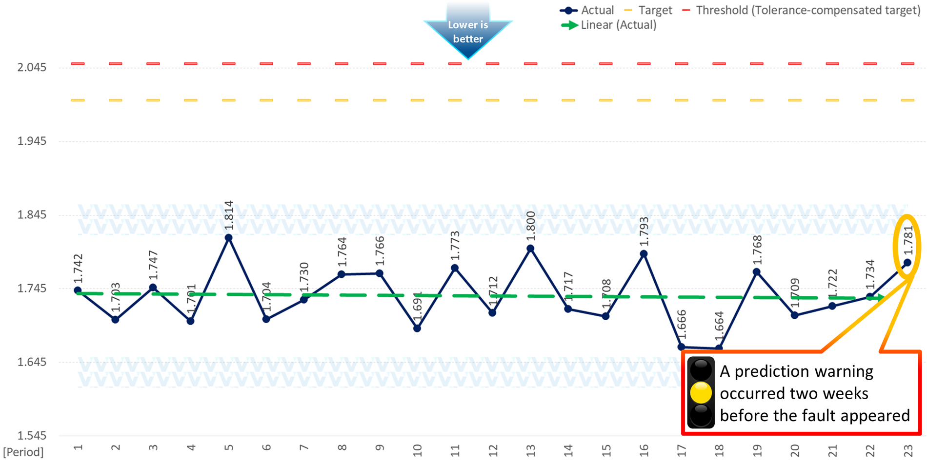
In the following real-life example, the system warns about wear caused by a friction problem occurring in the complex asset.
As a result, maintenance and replacement of malfunctioning components could be carried out without interrupting operation during runtime.
Based on daily measurements, the device is operating normally, and the linear trendline (green line) shows no change.
This indicator represents a ‘lower is better’ scenario, showcasing the power consumption of the electric engine.
In the 23rd period, an amber warning was issued because PRECOG detected an unusual operation.
The initial amber warning is followed by additional warnings every day, giving the maintenance personnel 2 weeks to perform the necessary inspections and ensure the delivery of required components.
Two weeks later, the warnings reach the red alert level, and on the following day, the maintenance personnel carry out the necessary maintenance and repairs before any faults could occur in the equipment.
From the 38th day onward, energy consumption returns to the normal operating range and the warnings will disappear.
In the following real-life example, the system warns about wear caused by a friction problem occurring in the complex asset.
As a result, maintenance and replacement of malfunctioning components could be carried out without interrupting operation during runtime.
Based on daily measurements, the device is operating normally, and the linear trendline (green line) shows no change.
This indicator represents a ‘lower is better’ scenario, showcasing the power consumption of the electric engine.
In the 23rd period, an amber warning was issued because PRECOG detected an unusual variation.
The initial amber warning is followed by additional warnings every day, giving the maintenance personnel 2 weeks to perform the necessary inspections and ensure the delivery of required components.
Two weeks later, the warnings reach the red alert level, and on the following day, the maintenance personnel carry out the necessary maintenance and repairs before any faults could occur in the equipment.
From the 38th day onward, energy consumption returns to the normal operating range and the warnings will disappear.
Further prediction examples
Short-Term Instant Fault Detection:
How PRECOG Spots Hidden Risks in Real Time
Medium-Term Predictive Motor Maintenance:
Stay Ahead of Malfunctions
Medium-term prediction example
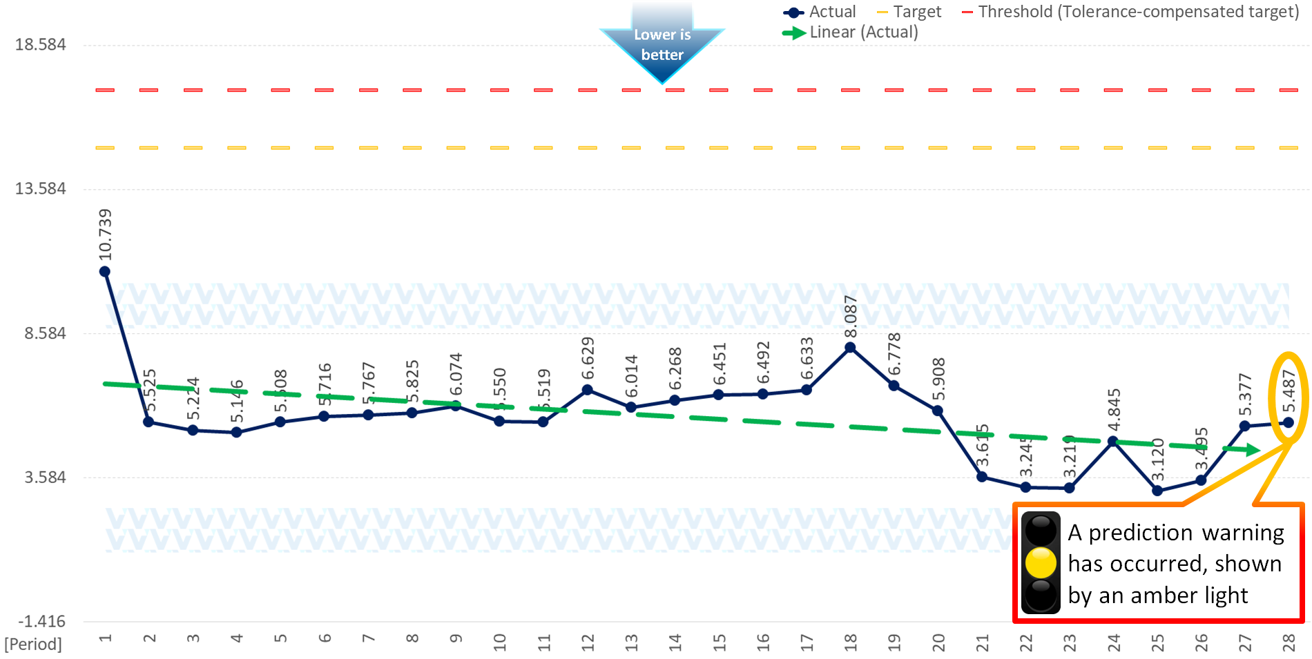
The following real-life example demonstrates a malfunction in a powerful electric motor, the consequences of which were mitigated thanks to the PRECOG predictive system, thereby maintaining operational safety without downtime.
This indicator represents a ‘lower is better’ scenario, showcasing the power consumption of the electric engine.
Each data point corresponds to the highest power consumption measured within every 4-hour interval.
Despite a negative trend (indicated by the green line), an amber prediction has been made.
Following the initial warning, two additional amber warnings were issued before a red alert was triggered.
Eventually, the power consumption exceeded the target threshold.
Consequently, competent specialists had ample time to prepare for the replacement of the critical engine with another device, thus preventing any downtime and damage to the affected equipment.
After repairs, the device could be put back into operation.
Short-term prediction example
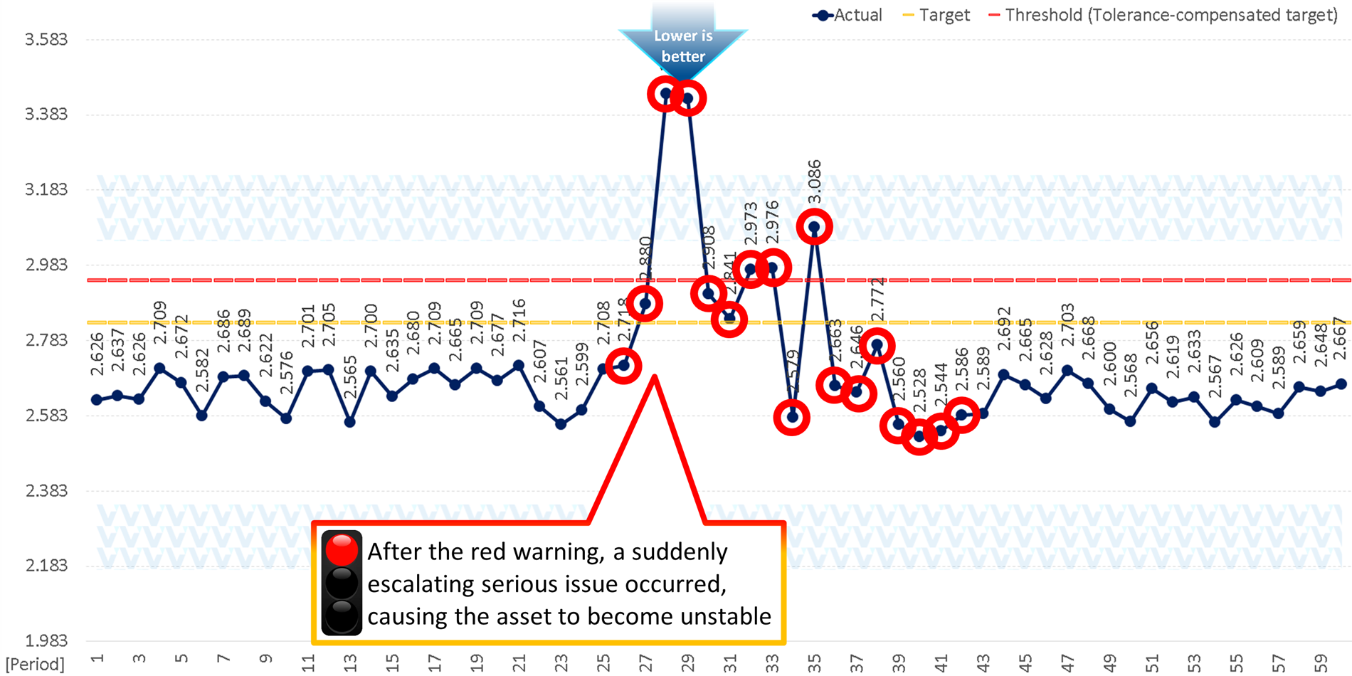
In the following real-life example, the system detected a suddenly arising serious fault.
The asset was operating within the usual range, and the linear trendline applied to the data (indicated by the green line) showed a very slight increase that did not indicate any problem.
This indicator represents a ‘lower is better’ scenario, showcasing the power consumption of the electric engine. Each data point corresponds to the highest power consumption measured within every 2-hour interval.
In the 26th period a red alert was received.
Following the red alert, the operator had approximately 4 hours to identify the causes of the suddenly appearing fault and to begin remediation.
Shutting down the asset, performing maintenance, or activating a backup system was not possible.
Shortly after the repairs, the system regained stability, which the operator was able to verify with the support of PRECOG, thus eliminating the need for further personal supervision.
Input file and what should the data contain?
Period
- This column signifies the timeframe during which the data was collected, arranged from the oldest to the most recent entries.
It can consist of numerical values or date/time stamps. - It's possible to aggregate the data to cover longer periods.
For example measurements taken every minute can be aggregated into days.
Whenever possible, this should be done at the raw data level. - Generally, we recommend using consistent time intervals such as days, hours, or minutes, which can then be aggregated for longer-term analysis.
- In special cases, such as with complex outdoor mechanical assets, where measurements may be particularly noisy and could mask underlying issues, please supply as many high-quality reference datasets as possible, ideally a minimum of 10 from any historical period.
Additionally, ensure that the last 6 records include the most recent values measured at consistent intervals or aggregated.
Actual
- This column represents the measured value of the asset or parameter being monitored.
The input file has to contain at least 6 records.
Target
- This column denotes the maximum or minimum threshold that the physical characteristic should not exceed, depending on the type of indicator.
For instance, in cases where a higher value is desirable, the target represents the maximum allowable value.
Conversely, if a lower value is preferable, the target represents the minimum acceptable value. - If the asset manufacturer does not specify the target, it is recommended to choose the target value based on test results so that it falls outside the upper and lower intervals marked in blue on the chart, thereby avoiding frequent alerts.
- The target can change throughout the entire period of the data and can affect the prediction.
Changes in the target can be used to represent the influence of other physical factors on the asset, such as temperature, rain, or other environmental effects.
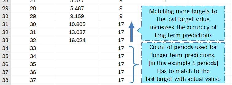
These adjustments are often applied to outdoor devices where different seasons and weather conditions may impact the asset. - The Target column is used to specify the count of periods required for longer-term predictions.
This can optionally be achieved by adding the desired periods with target values and tolerances without actual values.
Our recommendation is between 6 and 10 periods.
We do not recommend to exceed 14 periods, because the uncertainty factor increases exponentially, meaning that beyond 14, the accuracy of predictions will decrease significantly.
Any additional target values must match the target value corresponding to the last actual measured value.
Moving backward through the periods, the more target values match the last target value, the more accurate the long-term forecast will be.
Tolerance
- This column specifies the permissible deviation from the target value.
It represents a narrow threshold within which the equipment will continue to operate, but beyond which the operation may cause damage.
The tolerance value is either added to or subtracted from the target value, depending on whether the indicator type is 'Higher is better' or 'Lower is better'.
Higher is better
- This column is a binary indicator, denoted by either TRUE or FALSE, depending on the nature of the indicator.
If a higher value signifies better performance (also referred to as 'Green-Yellow-Red' or GYR), the column should be set to TRUE.
Conversely, if a lower value indicates superior performance (also known as 'Red-Yellow-Green' or RYG), the column should be set to FALSE.
Review and evaluation of the results
Lamp
The most important indicator result of the analysis is represented by the lamp.
It shows the summary analysis result of more than 14 different algorithms which can predict warnings or indicate critical alerts for the indicator.
Further information can be found in the details section.
Longer-term prediction
Longer-term prediction utilizes various prediction algorithms to estimate the overall performance probability of an indicator over an extended period.
In contrast, short-term prediction relies on a multitude of algorithms, hence the lamp providing appropriate predictions due to its utilization of numerous prediction algorithms.
Longer-term prediction assesses the probability of an indicator's performance even if it hasn't yet been fulfilled. The number of periods for long-term prediction can be adjusted based on the target set.
In general, the risk of non-performing is high below 70%.
Frequently Asked Questions
How is our solution any different from a standard predictive AI solution?
To put it simply, our AI has been fed with millions of records of real-life data from different industries over the course of 7 years and is powered by advanced mathematics.
How many records does Precog need to successfully do the evaluation being done?
We have a target. What does Tolerance do? What’s the difference?
My equipment has several data types. How will that be evaluated?
The algorithm runs on 1 data type at once. The best practice is to run the algorithm to each data type, and if any will return a yellow or red traffic light, the entire evaluation is considered to be either yellow or red. To represent the effect of different physical aspects (e.g.seasons, rain, temperature), target can be changed. This make sense mostly for outdoor devices.
How is the period measured? weeks, days, hours, minutes, etc?
Can I use different time measurements in an evaluation? for example, the first 10 values are in months, then next 10 are in weeks, then the last 10 in days?
Generally, we recommend using consistent time intervals such as days, hours, or minutes, which can then be aggregated for longer-term analysis.
Additionally, ensure that the last 6 records include the most recent values measured at consistent intervals or aggregated.
How long does it take for clients to be able to utilize and benefit from the Precog solution.
Typically the project takes around 2-4 months / equipment type.
This means that if you are on the lowest maturity scale and you want to get to the highest.
Once it’s rolled out, there is another 2 months observation / adjustment phase.


